
temperature restrict targets of 1.5°C by the tip of the century set by the Paris Settlement, totally different establishments have give you totally different situations. There’s a consensus amongst the mitigation scenarios that the share of low-carbon applied sciences comparable to renewable power wants to extend, and fossil fuels want to say no steadily within the power mixture of tomorrow.
The deployment of mitigation know-how choices (comparable to renewable power, Electrical Automobiles (EVs), inexperienced hydrogen, and so forth.) give you their very own set of prices and advantages. The combo of renewable power and fossil fuels within the electrical energy technology portfolio of a rustic not solely determines the CO2 emissions however may affect the electrical energy value. On this submit, I’m going to debate how the electrical energy value is set in a wholesale electrical energy market by advantage order curve (primarily based on the idea of marginal prices or manufacturing), and the way the cost-effectiveness of decarbonisation alternatives in a rustic or area or an organisation may very well be assessed primarily based on marginal abatement prices curve. I’m going to make use of Python to assemble these two curves, and focus on the implementation alongside the way in which.
Let’s get began!
Advantage Order Curve
An electrical energy authority or a utility in a rustic might have competing energy vegetation of various sorts in its portfolio to supply electrical energy output to retailers. This is named a wholesale electricity market (often known as spot market). The price of producing electrical energy differs in keeping with the kind of energy plant. For instance, there’s zero or minimal value of electrical energy technology from photo voltaic PV or wind generators since they don’t require any fuels. Alternatively, energy vegetation primarily based on fossil fuels have larger working prices relying on the costs of fuels comparable to coal, oil, or fuel that’s combusted to generate electrical energy. Within the language of economics, the price of producing one extra unit of a product is named marginal cost of production.Within the energy system, obtainable energy vegetation within the portfolio are scheduled to be on-line primarily based on the ascending order of short-run marginal prices of manufacturing of electrical energy. This sequence is known as the advantage order. The ability vegetation with the bottom marginal prices are scheduled to fulfill demand first, adopted by the facility vegetation with larger marginal prices to optimise the electrical energy provide prices.
On this part, I’m going to implement the totally different steps to assemble the advantage order curve in Python and focus on how the advantage order units the wholesale electrical energy value.
Implementation
Let’s contemplate that there are energy vegetation of 9 sorts within the electrical energy portfolio of a rustic as proven within the checklist power_plants. These energy vegetation have to be organized in ascending order of marginal_costs. The information used on this instance are primarily based on my assumption and may be thought to be dummy datasets.
power_plants = ["Solar", "Wind", "Hydro", "Nuclear", "Biomass", "Coal", "Gas", "Oil", "Diesel"]

marginal_costs = [0, 0, 5, 10, 40, 60, 80, 120, 130]
First, I convert this knowledge right into a dataframe with power_plants in index and marginal_cost within the column. Subsequent, I iterate by the index of dataframe and ask the person to enter the obtainable capability of every energy plant. The obtainable capability of every energy plant is saved in a person variable utilizing the globals() technique as proven under.
Asking person enter for the obtainable capability of every energy plant kind utilizing for-loop and the globals() technique.
The entire obtainable capability within the portfolio of nation X sums to 1800 MW. Then, I create a brand new column known as Cumulative capability (MW), which is the cumulative sum of Accessible capability (MW) .
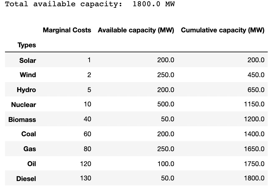
Dataframe containing marginal value and obtainable capability of every energy plant kind in nation X. Picture by Writer.
I ask the person to enter the electrical energy demand in nation X at a given timeframe.
demand = int(enter("Enter complete demand (MW): "))Let’s assume the demand is 1500 MW.
Now that the information is prepared, I can begin compiling the constructing blocks for the advantage order curve. In a advantage order curve, the facility plant are ordered in ascending order of marginal prices of electrical energy technology within the type of bar plots. The width of bars represents the obtainable capability of every energy plant kind and the peak represents the corresponding marginal value. For the reason that widths of bars usually are not equal, they give the impression of being fairly totally different from the traditional bar plots.
The place of ticks on the x-axis for the primary bar (right here Photo voltaic) is identical as half of its Accessible capability (MW). For the opposite energy plant kind, the place is calculated because the sum of Cumulative capability (MW) until the facility plant kind earlier than it, and half of its Accessible capability (MW). I’ve ready a for-loop to get this place in xpos column of df as proven within the first a part of the gist under.
Subsequent, I analyse the place at which the demand lies on the x-axis. The place at which the facility demand intersects with the cumulative energy provide on the x-axis determines cut_off_power_plant. In flip, the marginal value of the cut_off_power_plant determines the clearing value of all energy vegetation within the advantage order earlier than it, which take part within the wholesale market. The consumers of electrical energy on this wholesale market will all pay that very same value.
#For-loop to find out the place of ticks in x-axis for every bar
df["xpos"] = ""

for index in df.index:

    #get index quantity primarily based on index title
    i = df.index.get_loc(index)

    if index == "Photo voltaic":    #First index
        df.loc[index, "xpos"] = df.loc[index, "Available capacity (MW)"]

    else:
        #Sum of cumulative capability within the row above and the half of obtainable capability in
        df.loc[index, "xpos"] = df.loc[index, "Available capacity (MW)"]/2 + df.iloc[i-1, 2]


#Perform to find out the cut_off_power_plant that units the market clearing value
def cut_off(demand):
    #To get the cutoff energy plant
    for index in df.index:

        if df.loc[index, "Cumulative capacity (MW)"] < demand:
            move

        else:
            cut_off_power_plant = index
            print ("Energy plant that units the electrical energy value is: ", cut_off_power_plant)
            break

    return cut_off_power_plant
For loop on the highest determines the place of the bar of every energy plant kind on the x-axis. cut_off perform on the underside determines the facility plant kind that intersects with the facility demand.
The code to generate the advantage order curve is as proven.
def merit_order_curve(demand):
    plt.determine(figsize = (20, 12))
    plt.rcParams["font.size"] = 16

    colours = ["yellow","limegreen","skyblue","pink","limegreen","black","orange","grey","maroon"]
    xpos = df["xpos"].values.tolist()
    y = df["Marginal Costs"].values.tolist()
    #width of every bar
    w = df["Available capacity (MW)"].values.tolist()
    cut_off_power_plant = cut_off(demand)

    fig = plt.bar(xpos,
            peak = y,
            width = w,
            fill = True,
            colour = colours)

    plt.xlim(0, df["Available capacity (MW)"].sum())
    plt.ylim(0, df["Marginal Costs"].max() + 20)

    plt.hlines(y = df.loc[cut_off_power_plant, "Marginal Costs"],
              xmin = 0,
              xmax = demand,
              colour = "purple",
               linestyle = "dashed")

    plt.vlines(x = demand,
               ymin = 0,
               ymax = df.loc[cut_off_power_plant, "Marginal Costs"],
               colour = "purple",
               linestyle = "dashed",
               label = "Demand")

    plt.legend(fig.patches, power_plants,
              loc = "greatest",
              ncol = 3)

    plt.textual content(x = demand - df.loc[cut_off_power_plant, "Available capacity (MW)"]/2,
            y = df.loc[cut_off_power_plant, "Marginal Costs"] + 10,
            s = f"Electrical energy value: n    {df.loc[cut_off_power_plant, 'Marginal Costs']} $/MWh")

    plt.xlabel("Energy plant capability (MW)")
    plt.ylabel("Marginal Value ($/MWh)")
    plt.present()

merit_order_curve(demand = demand)
The ensuing plot is as proven under.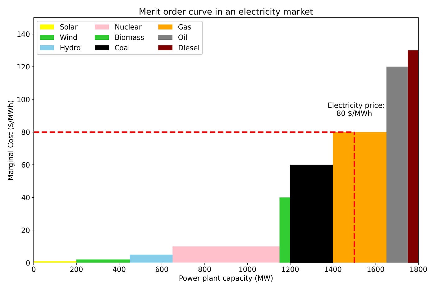 Advantage order curve of the given electrical energy market. The X-axis represents the obtainable capability of energy vegetation. The Y-axis represents the marginal value of every energy plant. The vertical purple dashed line represents the demand which is intersects with fuel. The horizontal dashed purple line represents the marginal value of electrical energy technology from fuel, which units the market clearing value. Picture by Writer.
Within the ensuing plot, the facility demand of 1500 MW is represented by the vertical dashed purple line. This coincides with the facility provide from fuel when all the facility vegetation are organized in ascending order by marginal value. Therefore, the marginal value of electrical energy technology from fuel i.e. 80 $/MWh is the market clearing value. This suggests all the facility vegetation on and earlier than the vertical dashed purple line on the X-axis i.e. photo voltaic, wind, hydro, nuclear, biomass, coal, and fuel have to ship energy to fulfill the demand. And all of them obtain the worth set by the marginal value of manufacturing from fuel.
Advantage Order Impact
When the demand stage modifications within the energy system, the wholesale electrical energy value additionally reacts accordingly. That is demonstrated within the GIF picture under. To get the animation in Python, I’ve used the work together perform from ipywidgets as proven under. I’ve additionally used IntSlider widget to set thedemand because the user-defined parameter to work together with. To keep away from flickering whereas dragging alongside the slider, I’ve set continuous_update to False.
from ipywidgets import *
demand = widgets.IntSlider(
                worth = 100,
                min = 0,
                max = df[“Available capacity (MW)”].sum(),
                step = 10,
                description = “Demand”,
                continuous_update = False #False to keep away from flickering
                )
interactive_plot = work together(merit_order_curve, demand = demand)
Animation displaying the change in reduce off energy plant and wholesale electrical energy value because the demand modifications. Picture by Writer.
As proven within the GIF picture above, when the demand will increase, extra energy vegetation in direction of the correct of the advantage order have to be dispatched, which will increase the clearing value and vice versa. If there’s a extra obtainable capability of renewable energy vegetation within the portfolio, extra share of the demand is met by renewable sources. This tends to decrease the electrical energy value, which is named the advantage order impact.
Marginal Abatement Value Curve
The abatement cost is a price borne by companies for eradicating or lowering the externalities (damaging byproducts) created throughout manufacturing. And the marginal abatement value measures the price of lowering one extra unit of externalities, e.g. CO2 emissions. Whereas the advantage order curve relies on ordering applied sciences by marginal prices of manufacturing, the marginal abatement prices (MAC) curve relies on ordering totally different mitigation alternatives within the ascending order of marginal abatement prices.
In a MAC curve, the width of the bar represents the greenhouse fuel (GHG) emissions discount potential of any know-how or possibility. And the peak of the bar represents the price of lowering one extra unit of GHG emissions with the given alternative. Dataframe containing mitigation potential and marginal abatement prices of various alternatives. Information relies on the writer’s assumption.
The information for this instance relies on my assumption and may be thought to be a dummy dataset. The implementation of the MAC curve in Python is much like that of the advantage order curve.
 MAC curve for a sure yr for nation X. Picture by Writer.
The width of the bar represents the annual GHG emissions discount potential of the mitigation alternative. The peak of the bar represents the estimated prices in a given yr to scale back emissions by 1 tCO2e.
As proven within the plot above, changing outdated lights with LED lights is probably the most cost-effective measure for decarbonisation. The damaging marginal abatement prices for sure alternatives suggest that there are web value financial savings (or revenue) when these measures are applied. As we transfer in direction of the correct finish of the X-axis in a MAC curve, it turns into costlier to abate one unit of GHG emissions. The widest bar on the MAC curve, reforestation has the best total potential of GHG emissions reductions.
Thus, the MAC curve permits measures from numerous sectors (right here energy, transport, buildings, forestry, and waste) to be in contrast on equal phrases. Whereas the MAC curve gives a key preliminary evaluation on the potential and cost-effectiveness of assorted mitigation alternatives, combining this evaluation with insights from different modelling instruments gives a robust base for formulating insurance policies and funding choices.
Conclusion
As we’re traversing by the worldwide power transition, burning extra fossil fuels to fulfill our power wants would result in quickly exceeding the emissions price range that we have to respect to fulfill the worldwide local weather goals. There are already technically confirmed and economically possible alternatives in place, that may considerably cut back GHG emissions from each power and non-energy sectors. Furthermore, with economies of scale, the confirmed mitigation applied sciences (e.g. wind and photo voltaic) are getting cheaper yearly.
You will need to harness the confirmed mitigation know-how choices to chop down on the emissions considerably. The mitigation choices give you their very own set of prices and advantages. On this submit, I mentioned how the share of renewable power and fossil fuels within the energy system portfolio of a rustic influences the wholesale electrical energy costs with the idea of advantage order curve (primarily based on marginal prices of manufacturing). And I introduced how the emissions discount potential and cost-effectiveness of mitigation alternatives in a rustic may very well be assessed primarily based on the marginal abatement value curve. The implementation of those curves in Python is on the market on this GitHub repository.